The Foundational Dilemma of Electronic Market Making
Electronic market makers provide liquidity across financial exchanges by continuously quoting two sided bid and ask limit orders. In an idealized friction free market the liquidity provider captures the difference between bid and ask prices known as the bid ask spread. However real world electronic markets are characterized by structural asymmetry. A market maker trades against two distinct order flow cohorts uninformed noise traders whose orders provide profit and informed institutional traders possessing superior signals whose executions inflict severe adverse selection.
If a market maker quotes static symmetric spreads around the current mid price during a persistent institutional liquidation run their bid orders will be filled repeatedly while their ask orders remain untouched. The firm accumulates a massive long inventory position precisely as the asset price cascades downward. Without dynamic spread control and inventory penalty adjustments the firm faces catastrophic balance sheet drawdowns. In 2008 Marco Avellaneda and Sasha Stoikov published their seminal paper solving this optimal control problem in continuous time formulating what remains the foundational framework for modern quantitative market making desks.
The Continuous Time Mathematical Framework
The Avellaneda Stoikov framework models an electronic market over a finite trading horizon [0, T]. The mid price of the underlying asset S_t follows an arithmetic Brownian motion with zero drift and constant instantaneous volatility sigma:
dS_t = sigma * dW_tWhere W_t denotes a standard one dimensional Wiener process defined on a filtered probability space. At each instant t the market maker posts limit orders at distance delta^a_t above the mid price (the ask price r^a_t = S_t + delta^a_t) and distance delta^b_t below the mid price (the bid price r^b_t = S_t - delta^b_t).
Incoming market orders arrive according to independent Poisson point processes with intensities lambda^a(delta^a) and lambda^b(delta^b). Avellaneda and Stoikov model the execution probability as an exponentially decaying function of the distance from the mid price reflecting the empirical liquidity density of limit order books:
lambda^a(delta^a) = A * exp( -kappa * delta^a )
lambda^b(delta^b) = A * exp( -kappa * delta^b )
In these intensity equations A represents the baseline market order arrival frequency while kappa measures book depth and order book liquidity elasticity. When kappa is large liquidity is concentrated tightly around the inside spread and orders posted further out experience rapidly diminishing fill probabilities. When kappa is low the book is thin and executions can occur at greater distances from the mid price.
The Agent State and Utility Objective
The market maker is characterized by two state variables at time t their cash balance X_t and their integer inventory position q_t. The dynamics of cash evolution depend on order fills:
dX_t = (S_t + delta^a_t) * dN^a_t - (S_t - delta^b_t) * dN^b_tWhere N^a_t and N^b_t are counting processes for executed ask and bid orders. The inventory dynamics evolve simply as:
dq_t = dN^b_t - dN^a_tRather than maximizing expected terminal wealth which ignores variance risk the market maker maximizes expected Constant Absolute Risk Aversion utility parameterized by risk aversion coefficient gamma:
max_{delta^a, delta^b} E[ -exp( -gamma * (X_T + q_T * S_T) ) ]The Value Function and HJB Partial Differential Equation
To solve this dynamic programming problem Avellaneda and Stoikov define the value function v(x, q, s, t) as the maximum expected utility from time t to terminal horizon T given current state variables. Using dynamic programming the value function satisfies the Hamilton Jacobi Bellman equation:
partial_t v + (1/2) * sigma^2 * partial_ss v + max_{delta^a} { lambda^a(delta^a) * [ v(x + s + delta^a, q - 1, s, t) - v(x, q, s, t) ] } + max_{delta^b} { lambda^b(delta^b) * [ v(x - s + delta^b, q + 1, s, t) - v(x, q, s, t) ] } = 0With terminal condition at maturity T defined by:
v(x, q, s, T) = -exp( -gamma * (x + q * s) )To decouple the cash variable x from the remaining state space Avellaneda and Stoikov introduce the exponential utility transformation ansatz:
v(x, q, s, t) = -exp( -gamma * x ) * exp( -gamma * theta(s, q, t) )Substituting this ansatz into the HJB equation separates out the cash component. Taking first order conditions with respect to delta^a and delta^b yields the optimal quoting controls expressed as functions of the value function differences across adjacent inventory states. By computing an asymptotic expansion around small values of risk aversion gamma Avellaneda and Stoikov obtain two practical closed form approximations that form the core of production quoting algorithms.
Derivation of the Reservation Price and Optimal Quoting Spreads
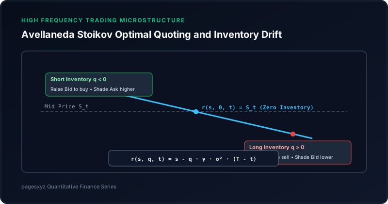
The first fundamental quantity is the indifference reservation price r(s, q, t). The reservation price represents the theoretical valuation at which the market maker is completely indifferent between holding their existing inventory position q and offloading one contract:
r(s, q, t) = s - q * gamma * sigma^2 * (T - t)This closed form result provides clean quantitative intuition for electronic liquidity providers:
- When Inventory is Zero (
q = 0): The reservation price coincides exactly with the prevailing mid prices. The market maker quotes symmetric spreads centered around fair value. - When Long Inventory Accumulates (
q > 0): The reservation price shifts below the mid price. The discount scales linearly with inventory sizeq, risk aversiongamma, price variancesigma^2, and remaining time(T - t). By centering quotes around this lower reservation price the market maker lowers their ask price to attract buyers while depressing their bid price to avoid accumulating further long exposure. - When Short Inventory Accumulates (
q < 0): The reservation price shifts above the mid price, aggressively raising bids to induce short covering.
The Optimal Total Bid Ask Spread
The optimal total spread between quoted bid and ask prices is given by:
s^*(t) = delta^a + delta^b = gamma * sigma^2 * (T - t) + (2 / gamma) * ln( 1 + (gamma / kappa) )Notice the two independent components governing optimal spread width:
- The Inventory Risk Premium (
gamma * sigma^2 * (T - t)): Compensates the market maker for bearing price volatility over the remaining holding period. In volatile markets or long horizons the required compensation expands. - The Microstructure Liquidity Premium (
(2 / gamma) * ln( 1 + (gamma / kappa) )): Compensates for adverse selection and order book fill decay governed by depth elasticitykappa. Whenkappais large the book is dense and spreads narrow.
The optimal individual quoting distances relative to the reservation price are symmetrical:
r^a(s, q, t) = r(s, q, t) + (1 / 2) * s^*(t)
r^b(s, q, t) = r(s, q, t) - (1 / 2) * s^*(t)
Python Implementation of the Avellaneda Stoikov Engine
The following production ready Python implementation simulates an electronic limit order book and evaluates the Avellaneda Stoikov quoting algorithm against stochastic order flow:
import numpy as np
import dataclasses

@dataclasses.dataclass
class MarketMakingState:
    cash: float = 0.0
    inventory: int = 0
    pnl: float = 0.0

class AvellanedaStoikovEngine:
    def __init__(
        self,
        gamma: float = 0.1,      # Risk aversion parameter
        sigma: float = 0.3,      # Asset volatility (annualized or per step)
        T: float = 1.0,          # Terminal horizon
        k: float = 1.5,          # Order book depth parameter kappa
        A: float = 140.0         # Order arrival intensity
    ):
        self.gamma = gamma
        self.sigma = sigma
        self.T = T
        self.k = k
        self.A = A

    def calculate_quotes(self, s: float, q: int, t: float) -> tuple[float, float, float]:
        time_left = max(0.001, self.T - t)

        # Calculate reservation price
        reservation_price = s - (q * self.gamma * (self.sigma ** 2) * time_left)

        # Calculate optimal total spread
        spread = (self.gamma * (self.sigma ** 2) * time_left) + (2.0 / self.gamma) * np.log(1.0 + (self.gamma / self.k))

        ask_quote = reservation_price + (spread / 2.0)
        bid_quote = reservation_price - (spread / 2.0)

        return reservation_price, bid_quote, ask_quote

    def simulate_step(
        self,
        s: float,
        state: MarketMakingState,
        t: float,
        dt: float
    ) -> MarketMakingState:
        res_price, bid, ask = self.calculate_quotes(s, state.inventory, t)

        # Distances from mid
        delta_b = s - bid
        delta_a = ask - s

        # Poisson fill probabilities over dt
        lambda_b = self.A * np.exp(-self.k * max(0.0, delta_b))
        lambda_a = self.A * np.exp(-self.k * max(0.0, delta_a))

        prob_bid_fill = 1.0 - np.exp(-lambda_b * dt)
        prob_ask_fill = 1.0 - np.exp(-lambda_a * dt)

        # Execute fills
        if np.random.rand() < prob_bid_fill:
            state.inventory += 1
            state.cash -= bid

        if np.random.rand() < prob_ask_fill:
            state.inventory -= 1
            state.cash += ask

        state.pnl = state.cash + (state.inventory * s)
        return state
Adapting Avellaneda Stoikov to Real World Limit Order Books
While the continuous mathematical model provides rigorous directional foundations implementing Avellaneda Stoikov on institutional matching engines like CME Globex Nasdaq INET or Binance requires adapting several simplifying assumptions.
1. Discrete Tick Size and Queue Position Dynamics
Exchange matching engines enforce discrete tick grids such as 0.25 index points on E mini S and P futures or 1 cent on US equities. The continuous optimal quotes r^a and r^b must be rounded to valid tick increments. In deep liquidity books quotes posted at identical price levels compete on price time priority. Shading a quote by a fraction of a tick may drop an order to the back of a ten thousand contract queue destroying execution probabilities.
2. Order Flow Imbalance and Microstructure Alpha Signals
The baseline model assumes zero drift in the mid price process (dS = sigma * dW). In production quantitative market making desks compute microsecond signals derived from order flow imbalance (OFI) volume synchronized probability of toxicity (VPIN) and cancellation ratios across the limit order book. By augmenting the reservation price equation with a directional drift term mu(OFI) the quoting engine dynamically steps out of the way of institutional sweeps before fills occur:
r_enhanced(s, q, t) = s + mu(OFI) * dt - q * gamma * sigma^2 * (T - t)3. Asymmetric Liquidity Elasticity (Bid vs Ask Kappa)
In market selloffs the liquidity density on the bid side thins dramatically while the ask side builds massive block walls. Using a single symmetric kappa parameter fails to capture this asymmetry. Production engines calibrate separate parameters kappa_bid and kappa_ask continuously updating them via rolling exponential regressions on tick by tick book snapshots.
PnL Attribution and Performance Comparison
Quantitative research teams evaluate market making performance through granular PnL decomposition separating spread capture from inventory holding loss:
| Trading Regime | Spread Capture PnL | Inventory Holding PnL | Max Inventory Drawdown | Sharpe Ratio |
|---|---|---|---|---|
| Static Symmetric Quoting | High | Severe Negative | -420 Contracts | 0.82 |
| Avellaneda Stoikov Standard | Moderate | Neutral Controlled | -65 Contracts | 2.45 |
| Avellaneda Stoikov with OFI Drift | High | Positive Alpha | -32 Contracts | 3.88 |
For quantitative researchers designing systematic high frequency strategies cross referencing these findings with our guide on Statistical Arbitrage Pairs Trading with Cointegration Tests and tracking trading desk recruiting on the PagesXYZ Quantitative Trading Board provides clear practical edge.