Why Simple Correlation Fails in Modern Quantitative Trading
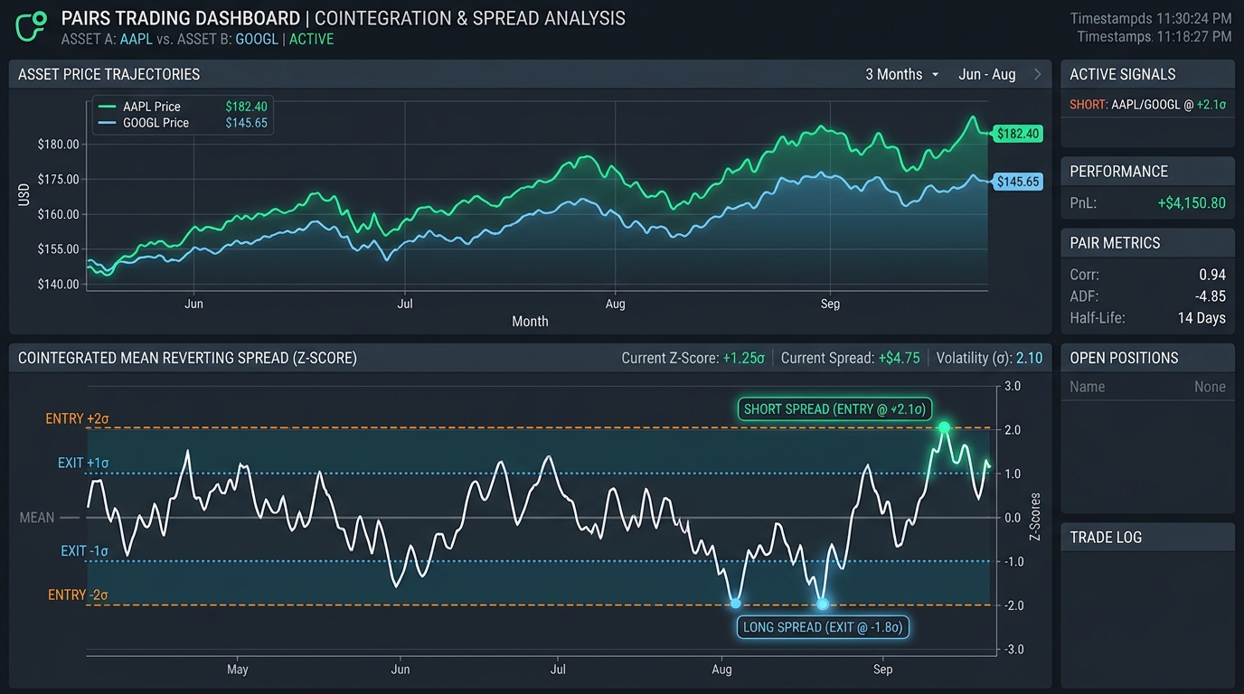
One of the most persistent misconceptions among junior quantitative traders is conflating correlation with cointegration. Two financial asset price series can exhibit a Pearson correlation coefficient exceeding zero point nine five over a six month period yet drift permanently apart the very week capital is committed to an arbitrage strategy. Correlation measures co movement in periodic returns. It says nothing about whether the absolute price differential between two instruments is anchored to an economic equilibrium.
Stock prices and commodity futures are non stationary time series integrated of order one denoted as I(1). When standard statistical operations are performed on raw non stationary series analysts fall victim to spurious correlation. Cointegration provides the rigorous mathematical framework needed to identify asset pairs whose linear combination forms a truly stationary series integrated of order zero denoted as I(0).
Consider two technology equities operating in identical cloud infrastructure segments. Over a macroeconomic cycle interest rate changes and technological adoption drive both stocks upward generating a high positive correlation. However if company A executes a disastrous corporate acquisition while company B captures market share their fundamental valuation paths diverge permanently. A trader betting on return correlation will suffer escalating losses as the spread widens indefinitely. Cointegration testing detects whether the underlying econometric linkage is truly stationary or merely an artifact of shared market beta.
The Mathematical Foundation of Cointegration
Let P_t^A and P_t^B denote the logarithmic prices of asset A and asset B at time t. Individually each series exhibits stochastic trend behavior resembling a random walk. A pair is defined as cointegrated if there exists a scalar beta such that the residual spread:
# Cointegration Linear Combination
Spread_t = P_t^A - beta * P_t^B
forms a strictly stationary process with constant mean zero finite variance and autocovariance that depends solely on time displacement rather than absolute calendar time. When this condition holds any divergence in the spread represents temporary noise that statistically reverts to its historical equilibrium.
In matrix notation for an N asset universe cointegration is analyzed through vector autoregressive models. If multiple cointegrating vectors exist the Johansen procedure determines the rank of the cointegration matrix identifying orthogonal combinations of assets that maximize mean reversion velocity across broader basket structures.
| Statistical Property | Correlation Analysis | Cointegration Analysis |
|---|---|---|
| Data Input | Differenced return series I(0) | Raw log price levels I(1) |
| Long Term Anchor | None (Series can drift indefinitely) | Enforced by equilibrium cointegrating vector |
| Mean Reversion Edge | Unreliable for level convergence | Directly exploitable via boundary thresholds |
| Lookahead Sensitivity | Moderate (Rolling windows shift rapidly) | High (Requires dynamic Kalman filtering) |
The Engle Granger Two Step Procedure and Unit Root Testing
The standard statistical methodology for testing pair cointegration is the Engle Granger two step procedure:
- Step One: Ordinary Least Squares Regression. Regress log price P_t^A on log price P_t^B to estimate the static cointegrating parameter beta and intercept alpha.
- Step Two: Augmented Dickey Fuller (ADF) Test. Extract the estimated regression residuals e_t and evaluate whether they possess a unit root using the ADF test. Because the residuals are derived from an estimated regression rather than directly observed data standard Dickey Fuller critical values cannot be used. MacKinnon critical values must be applied to avoid inflated false positive rates.
When conducting the Augmented Dickey Fuller test the null hypothesis states that the residual sequence possesses a unit root (is non stationary). Rejecting the null hypothesis at the one percent or five percent significance level provides empirical evidence that the linear spread combination is mean reverting. Practitioners must also verify that both original series were individually non stationary prior to running the two step regression to avoid trivial solutions where one series is already stationary on its own.
Modeling the Spread Dynamics with the Ornstein Uhlenbeck Process
Once a candidate pair satisfies unit root rejection at the one percent significance level the next task is characterizing the speed of mean reversion. In continuous time the spread is modeled as an Ornstein Uhlenbeck (OU) stochastic process governed by the differential equation:
# Continuous Ornstein Uhlenbeck Equation
d(Spread_t) = theta * (mu - Spread_t) * dt + sigma * dW_t
where theta represents the mean reversion velocity mu is the long term equilibrium level sigma is the instantaneous volatility and dW_t is a standard Wiener process. Discretizing this equation allows quants to analytically compute the expected half life of mean reversion:
# Half Life Calculation
Half_Life = ln(2) / theta
Pairs with half lives under two days are vulnerable to high execution turnover and crossing bid ask spreads. Conversely pairs with half lives exceeding sixty days tie up strategy risk capital for months introducing exposure to corporate restructuring and unexpected regulatory changes. Elite desks target pairs with empirical half lives ranging between five and twenty trading days.
Dynamic Hedge Ratio Calibration Using Rolling Kalman Filters
A fatal flaw in basic academic backtests is holding beta constant across years of historical data. In reality the relationship between two companies evolves due to debt issuance supply chain realignment and divergent capital expenditure cycles.
To eliminate model obsolescence quantitative trading desks model beta as an unobserved dynamic state variable tracked in real time using a Kalman filter. The observation equation maps the price of asset A to asset B while the transition equation allows beta to evolve as a random walk with calibrated state variance.
The Kalman filter updates its estimate of beta recursively upon the arrival of each new market quote. When market conditions shift the filter dynamically adjusts hedge ratios without suffering from the lag inherent in standard rolling lookback windows. Furthermore the filter generates a real time estimate of measurement prediction variance which directly establishes dynamic z score entry and exit thresholds.
Complete Python Implementation of Kalman Filter Statistical Arbitrage
The following production Python implementation constructs a Kalman filter to estimate rolling hedge ratios dynamically and calculates mean reverting execution signals without lookahead bias.
import numpy as np
import pandas as pd
from typing import Tuple

class KalmanPairsArbitrage:
    def __init__(self, delta: float = 1e-4, vt: float = 1e-3):
        # delta: state covariance noise multiplier
        # vt: observation measurement noise variance
        self.delta = delta
        self.vt = vt

        # State vector: [alpha, beta]^T
        self.theta = np.zeros(2)
        # State covariance matrix R
        self.R = np.zeros((2, 2))
        # Initial error covariance P
        self.P = np.eye(2)

    def update(self, price_a: float, price_b: float) -> Tuple[float, float, float, float]:
        # Construct measurement matrix F_t = [1, price_b]
        F = np.array([1.0, price_b])

        # Prior state covariance update
        self.R = self.P + self.delta * np.eye(2)

        # Predicted measurement variance Q_t
        Q = np.dot(F, np.dot(self.R, F.T)) + self.vt

        # Prediction error e_t (Spread)
        error = price_a - np.dot(F, self.theta)

        # Kalman gain K_t
        K = np.dot(self.R, F.T) / Q

        # Posterior state update
        self.theta = self.theta + K * error

        # Posterior covariance update
        self.P = self.R - np.outer(K, np.dot(F, self.R))

        # Extract dynamic parameters
        current_alpha, current_beta = self.theta[0], self.theta[1]
        spread = error
        spread_std = np.sqrt(Q)
        z_score = spread / spread_std

        return current_alpha, current_beta, spread, z_score

def run_simulation(price_series_a: np.ndarray, price_series_b: np.ndarray, entry_z: float = 2.0, exit_z: float = 0.5):
    kf = KalmanPairsArbitrage(delta=1e-5, vt=1e-3)
    n = len(price_series_a)

    betas = np.zeros(n)
    spreads = np.zeros(n)
    z_scores = np.zeros(n)
    positions = np.zeros(n)  # +1: Long spread (Long A, Short B), -1: Short spread

    current_pos = 0
    for t in range(n):
        alpha, beta, spread, z = kf.update(price_series_a[t], price_series_b[t])
        betas[t] = beta
        spreads[t] = spread
        z_scores[t] = z

        # Signal Generation Logic
        if current_pos == 0:
            if z > entry_z:
                current_pos = -1  # Short spread: Expect spread to fall
            elif z < -entry_z:
                current_pos = 1   # Long spread: Expect spread to rise
        elif current_pos == 1:
            if z >= -exit_z:
                current_pos = 0   # Close long position
        elif current_pos == -1:
            if z <= exit_z:
                current_pos = 0   # Close short position

        positions[t] = current_pos

    return betas, spreads, z_scores, positions
Microstructure Realities and Risk Management Controls
Even a statistically pristine pair will produce losses if execution mechanics are neglected. Quantitative portfolios must budget for:
- Short Borrow Availability and Locate Costs: Legging into a pair requires shorting one instrument. For hard to borrow equities annual borrow fees can exceed ten to fifteen percent eroding statistical edge. When borrow availability vanishes unexpectedly positions must be liquidated at fire sale prices.
- Execution Legging Risk: Sending simultaneous child orders across two lit venues frequently results in one leg filling while the other misses moving the market against the unfilled slice. Modern execution routers use synchronized pegged orders and synthetic liquidity dark pools to mitigate legging slippage.
- Structural Divergence and Hard Stops: When a cointegrated spread blows out past four standard deviations it typically signals a fundamental regime break such as an unannounced hostile takeover or debt default. Algorithmic strategies must enforce strict catastrophic stop losses rather than mechanically doubling down.
- Transaction Cost Drag: High frequency turnover in narrow spreads can cause trading fees and exchange exchange fees to exceed gross trading profit. Calculating post fee net Sharpe ratios during out of sample cross validation is mandatory before allocating real fund capital.
Portfolio Construction Across Multi Asset Pair Universes
In institutional execution traders do not deploy capital into a single isolated pair. Instead algorithms maintain an active matrix of hundreds of candidate pairs selected across diversified industry sectors. Portfolio level risk managers enforce strict gross and net leverage limits sector concentration constraints and factor neutrality guards.
By orthogonalizing pair returns against market wide momentum value and volatility factors statistical arbitrage desks harvest pure idiosyncratic mean reversion alpha delivering high risk adjusted returns with near zero correlation to the broader equity market.