The Mechanics of Post Training Alignment in Frontier LLMs
Post training has superseded raw pretraining as the primary locus of capability differentiation in frontier artificial intelligence architectures. While next token prediction over petabyte scale corpora builds foundational representations of syntax world knowledge and algorithmic reasoning it leaves foundation models poorly calibrated for instruction following complex tool execution and multi turn safety. Alignment bridges this gap by conditioning generation probabilities on human and automated preferences.
Historically the dominant methodology for preference alignment was Reinforcement Learning from Human Feedback known as RLHF operationalized through Proximal Policy Optimization. PPO adapts policy gradients from continuous control robotics to discrete token decoding spaces. However scaling PPO to models with seventy billion or hundreds of billions of parameters introduces severe systems friction. Training instability hyperparameter sensitivity and massive GPU memory overhead have driven frontier laboratories to seek alternative closed form formulations. Direct Preference Optimization emerged as the preeminent alternative eliminating intermediate reward models and actor critic value heads entirely.
Understanding the exact mathematical derivations systemic trade offs and failure modes between PPO and DPO is essential for machine learning systems engineers. Both approaches optimize under identical theoretical constraints yet their execution characteristics on Hopper and Blackwell GPU clusters diverge dramatically.
The Classical PPO Alignment Pipeline and Its Scaling Bottlenecks
The standard RLHF pipeline under Proximal Policy Optimization consists of three distinct phases. First a pre trained model undergoes supervised fine tuning on high quality demonstration pairs. Second a scalar reward model is trained on pairwise comparison datasets where annotators or synthetic judges score preferred completions over rejected alternatives under the Bradley Terry preference model. Third the supervised policy acts as an agent in a Markov Decision Process where generating a full sequence corresponds to a trajectory and the reward model evaluates terminal state value.
The mathematical objective function that PPO attempts to maximize balances reward maximization against policy drift via a Kullback Leibler divergence penalty:
max_theta E_{x ~ D, y ~ pi_theta(y|x)} [ r_psi(x, y) - beta * D_KL( pi_theta(y|x) || pi_ref(y|x) ) ]Here r_psi(x, y) represents the scalar output of the frozen reward model parameterized by weights psi while pi_ref is the frozen reference policy matching the supervised initialization. The parameter beta controls the regularization strength preventing the policy pi_theta from collapsing into degenerate distribution modes that exploit reward model misspecification also known as reward hacking.
The Four Model Memory Tax in GPU VRAM
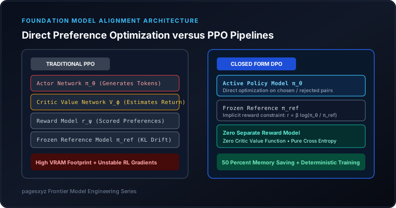
The principal operational limitation of PPO lies in its physical memory layout. At any instant during training a production PPO worker must maintain four distinct model weight sets across its distributed tensor and pipeline parallel groups:
- The Active Actor Policy (
pi_theta): The model receiving gradient updates requiring optimizer states Adam momentum and variance buffers and backward activations. - The Critic Value Network (
V_phi): A separate transformer backbone estimating token level expected future returns required for Generalized Advantage Estimation. - The Frozen Reward Model (
r_psi): A sequence classification transformer scoring generated candidate completions. - The Frozen Reference Policy (
pi_ref): An identical copy of the actor network evaluated in inference mode to compute token level KL divergence penalties.
For a 70B parameter model in 16 bit floating point representation each model instance requires approximately 140 gigabytes of VRAM purely for static weights. With Adam optimizer states requiring 16 bytes per parameter for FP32 master weights and momentum terms the actor policy alone consumes roughly 1.1 terabytes of memory before accounting for activations and KV cache buffers during trajectory generation. Coordinating inference generation across the actor model followed by value prediction on the critic and scoring on the reward model creates severe distributed pipeline bubbles and stalls.
Mathematical Derivation of Closed Form Direct Preference Optimization
Direct Preference Optimization introduced by Rafailov and colleagues bypasses the reinforcement learning framing entirely by reparameterizing the reward function directly through the language model policy. The insight stems from recognizing that the constrained optimization problem solved by PPO has an exact analytical solution.
Recall the constrained objective under a prompt distribution D. By applying calculus of variations to the Lagrangian of the expected reward with KL regularization we obtain the closed form expression for the optimal policy pi^*:
pi^*(y|x) = (1 / Z(x)) * pi_ref(y|x) * exp( (1 / beta) * r(x, y) )In this relationship Z(x) is the per prompt partition function normalizing the probability distribution across all possible generated sequences:
Z(x) = sum_y pi_ref(y|x) * exp( (1 / beta) * r(x, y) )Crucially we can algebraically invert this formulation to express the ground truth reward function r(x, y) strictly in terms of the optimal policy the reference policy and the partition function:
r(x, y) = beta * ln( pi^*(y|x) / pi_ref(y|x) ) + beta * ln( Z(x) )Substitution into the Bradley Terry Preference Formulation
We assume that preference datasets consist of triples containing a prompt x a preferred chosen response y_w and a dispreferred rejected response y_l. Under the Bradley Terry model the probability that a judge prefers completion y_w over y_l depends exclusively on the sigmoid of their reward differential:
P(y_w > y_l | x) = sigma( r(x, y_w) - r(x, y_l) )When we substitute our inverted reward expression into this preference likelihood a mathematical cancellation occurs. The prompt dependent partition term beta * ln( Z(x) ) appears identically in both reward evaluations and subtracts out completely:
r(x, y_w) - r(x, y_l) = beta * ln( pi_theta(y_w|x) / pi_ref(y_w|x) ) - beta * ln( pi_theta(y_l|x) / pi_ref(y_l|x) )This cancellation eliminates the intractable sum over all token sequences. Taking the negative log likelihood over the empirical preference dataset yields the exact DPO loss function:
L_DPO(theta; pi_ref) = - E_{(x, y_w, y_l) ~ D} [ ln sigma( beta * ln( pi_theta(y_w|x) / pi_ref(y_w|x) ) - beta * ln( pi_theta(y_l|x) / pi_ref(y_l|x) ) ) ]Because this loss is fully differentiable with respect to theta model weights can be trained using standard cross entropy backpropagation without sampling tokens on the fly without training a separate critic network and without evaluating an external reward model.
PyTorch Reference Implementation of the DPO Loss Function
To inspect how this analytical loss operates in production consider the following PyTorch implementation designed for distributed model training:
import torch
import torch.nn as nn
import torch.nn.functional as F

class DirectPreferenceOptimizationLoss(nn.Module):
    def __init__(self, beta: float = 0.1, label_smoothing: float = 0.0):
        super().__init__()
        self.beta = beta
        self.label_smoothing = label_smoothing

    def forward(
        self,
        policy_chosen_logps: torch.FloatTensor,
        policy_rejected_logps: torch.FloatTensor,
        reference_chosen_logps: torch.FloatTensor,
        reference_rejected_logps: torch.FloatTensor
    ) -> tuple[torch.Tensor, torch.Tensor, torch.Tensor]:
        # Calculate log ratios between active policy and reference policy
        chosen_logratios = policy_chosen_logps - reference_chosen_logps
        rejected_logratios = policy_rejected_logps - reference_rejected_logps

        # Scale by regularization hyperparameter beta
        logits = self.beta * (chosen_logratios - rejected_logratios)

        if self.label_smoothing > 0.0:
            loss = (
                -F.logsigmoid(logits) * (1.0 - self.label_smoothing)
                - F.logsigmoid(-logits) * self.label_smoothing
            ).mean()
        else:
            loss = -F.logsigmoid(logits).mean()

        # Implicit rewards for telemetry and monitoring
        chosen_rewards = self.beta * chosen_logratios.detach()
        rejected_rewards = self.beta * rejected_logratios.detach()

        return loss, chosen_rewards, rejected_rewards
Notice the simplicity of this loss tensor computation. The inputs are simply the sequence summed log probabilities of the target tokens evaluated under the active model and the frozen reference model. During a training batch both chosen and rejected sequences are forwarded through the network in standard teacher forcing mode.
Failure Modes Likelihood Displacement and Length Bias in DPO
Despite its mathematical elegance DPO exhibits several distinct failure modes that have been uncovered across empirical deployments in frontier research laboratories.
1. Implicit Likelihood Displacement
Because the DPO objective depends strictly on the difference between chosen and rejected log ratios the loss function can be minimized without increasing the absolute probability of the chosen response. In practice if the active policy aggressively depresses the log likelihood of the rejected sequence pi_theta(y_l|x) faster than it decreases pi_theta(y_w|x) the loss still declines.
This dynamic leads to likelihood displacement where both chosen and rejected sequences experience declining probability density over prolonged training steps. In extreme cases this degradation damages the base capabilities of the model causing grammatical degeneration repetitive phrasing and token hallucinations.
2. Severe Length and Verbosity Exploitation
Preference datasets curated by human annotators frequently contain systemic biases. Humans systematically rate longer more elaborately formatted responses as higher quality even when the underlying reasoning is redundant or incorrect. When DPO optimizes over log likelihoods summed across variable token lengths longer sequences accumulate larger cumulative log ratios.
Frontier models fine tuned with basic DPO rapidly exhibit verbosity bloat producing answers three to five times longer than necessary to maximize implicit margin scores. Counteracting this requires length normalized implicit rewards or regularized loss variants like Simple Preference Optimization known as SimPO.
Architectural Comparison across Key Engineering Metrics
The choice between PPO and DPO involves fundamental engineering trade offs spanning hardware efficiency training dynamics and sample efficiency. The following comparison summarizes these properties:
| Engineering Dimension | Proximal Policy Optimization (PPO) | Direct Preference Optimization (DPO) |
|---|---|---|
| Active GPU Memory Models | 4 Models (Actor Critic Reward Reference) | 2 Models (Actor Policy and Reference Policy) |
| Training Regime | On policy reinforcement learning | Offline supervised contrastive learning |
| Online Sequence Generation | Mandatory during training loop | Zero token generation required |
| Hyperparameter Sensitivity | Extreme (GAE lambda clipping ratios learning rates) | Moderate (primarily regularization factor beta) |
| Wall Clock Training Speed | 3x to 5x slower due to generation phase | Fast matching standard SFT training throughput |
| Susceptibility to OOD Exploits | High via reward model hacking | Moderate via likelihood displacement |
| Cluster Scaling Complexity | High requires complex Megatron pipeline layout | Low scales cleanly with standard FSDP or ZeRO |
Production Deployment and Frontier Recommendations
For modern production alignment pipelines DPO represents the superior default choice for standard conversational instruction tuning coding assistance and style adherence. By eliminating the critic network and real time token generation loops engineering teams can align models twice as large on existing GPU compute budgets.
However when engineering complex multi step reasoning agents targeting competitive mathematics or autonomous software development PPO and its modern online variants like Group Relative Policy Optimization retain distinct advantages. Online RL allows models to explore trajectories not present in static offline preference datasets enabling true test time compute scaling and self correction. Teams evaluating frontier engineering trade offs should inspect our companion study on Scaling Laws for Autoregressive Reasoning and Test Time Compute and explore career openings across leading research labs on the PagesXYZ Engineering Board.