The Confounder Trap in Standard Machine Learning
Modern machine learning models excel at predictive accuracy. Given a high dimensional feature vector an ensemble of gradient boosted trees or a multi layer neural network can estimate consumer purchase probability with exceptional precision. However in strategic business decision making prediction is fundamentally insufficient. Executives and system architects must understand causation: If we raise software subscription fees by twelve percent what will happen to net revenue? If we inject a new promotional banner into the checkout workflow what is the true incremental conversion lift?
When analysts fit standard supervised learning models directly to observational historical data they encounter severe confounding bias. For example high volume enterprise users might naturally adopt a premium platform feature without any marketing encouragement while simultaneously maintaining lower churn rates. A naive regression will attribute customer retention to feature usage when both were actually caused by company size. In econometric terminology the feature treatment variable is endogenous.
Traditional data science workflows often attempt to resolve confounding by running randomized controlled trials (A/B tests). However randomized experimentation is frequently expensive risky or ethically impractical. In financial credit risk pricing decisions or patient healthcare treatment analysis models must extract reliable causal parameters from vast repositories of observational historical data without inducing catastrophic policy errors.
The Frisch Waugh Lovell Theorem and Modern Semi Parametric Inference
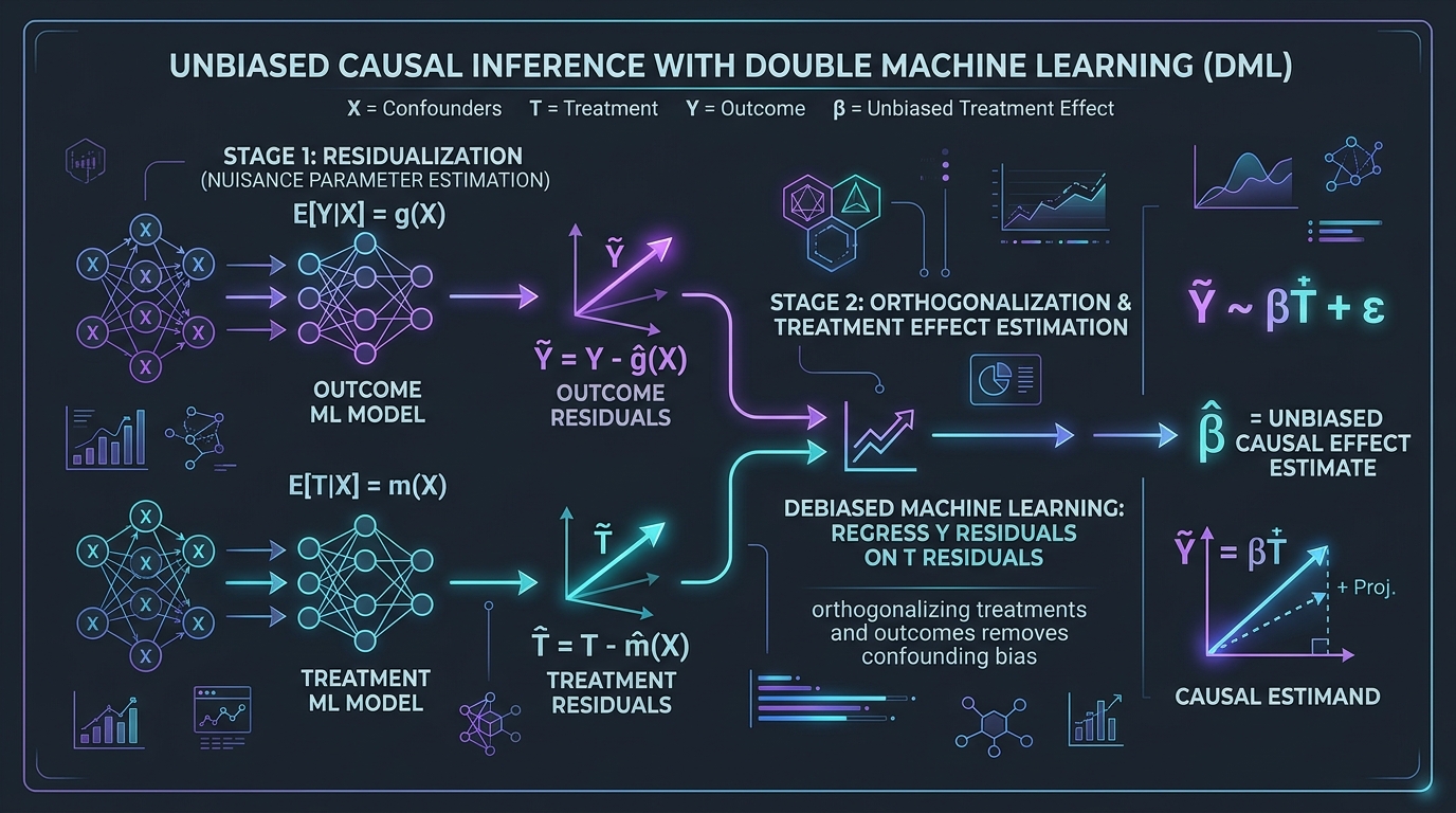
To isolate the true causal impact of a treatment variable T on an outcome Y in the presence of confounding covariates X economists historically relied on the Frisch Waugh Lovell (FWL) theorem. The theorem proves that in linear models the regression coefficient of T can be obtained by a two stage procedure:
- Regress outcome Y on covariates X and compute the residual outcome.
- Regress treatment T on covariates X and compute the residual treatment.
- Regress the residual outcome on the residual treatment to estimate the unbiased treatment effect.
While elegant the classical FWL theorem assumes strictly linear relationships between covariates and outcomes. In modern production environments where feature matrices contain thousands of customer telemetry attributes linear approximations break down. Complex non linear interactions between user age engagement frequency and historical billing render standard linear regressions misspecified.
Neyman Orthogonality and Double Robustness
A natural temptation is to replace simple linear regressions with flexible machine learning algorithms like LightGBM or Random Forests in the residualization step. However doing so naively introduces a subtle mathematical failure known as regularization bias. High capacity machine learning models employ regularization penalties (such as L1 Lasso or tree depth constraints) to prevent overfitting. This regularization systematically shrinks estimated nuisance parameters introducing first order bias into the target causal estimand.
Double Machine Learning (DML) developed by Chernozhukov and colleagues resolves this dilemma by constructing a score function that satisfies Neyman Orthogonality. A score function is Neyman orthogonal if its Gateaux derivative with respect to the nuisance functions vanishes at the true parameter values. This mathematical guarantee ensures that errors in predicting the nuisance components have only a negligible second order impact on the estimated treatment parameter.
| Methodology | Covariate Handling | Regularization Bias | Asymptotic Normality |
|---|---|---|---|
| Naive OLS | Linear assumptions only | None (Unregularized) | Severely biased if non linear |
| Standard ML Regression | Arbitrary non linear interactions | High first order bias | Invalid confidence intervals |
| Double Machine Learning | Arbitrary ML algorithms | Zero first order bias | Root N consistency and valid inference |
| Propensity Score Matching | Dependent on overlap | Moderate curse of dimensionality | Sensitive to common support boundary |
The Vital Role of Sample Splitting and K Fold Cross Fitting
Alongside Neyman orthogonality Double Machine Learning enforces a second strict requirement: cross fitting. If the same training observations are used both to estimate the nuisance parameters and to compute the final causal coefficient stochastic dependencies between the residuals violate Donsker empirical process conditions.
Cross fitting partitions the dataset into K out of sample folds. When evaluating residuals for fold K the nuisance models are trained exclusively on the remaining K minus one folds. Cycling through all folds produces out of sample residual vectors across the entire population completely eliminating in sample overfitting bias.
Because the nuisance estimators converge at a relatively slow non parametric rate (such as N to the power of negative one quarter) standard estimators would fail to achieve asymptotic normality. Thanks to the twin pillars of Neyman orthogonality and cross fitting the final causal parameter converges at the parametric root N rate allowing quants and data scientists to construct valid confidence intervals and perform hypothesis testing.
Complete Python Implementation of a Production Double ML Estimator
Below is a clean modular Python implementation demonstrating an end to end Double Machine Learning estimator with K fold cross fitting.
import numpy as np
from sklearn.model_selection import KFold
from sklearn.ensemble import GradientBoostingRegressor
from typing import Dict, Any

class DoubleMachineLearningEstimator:
    def __init__(self, n_splits: int = 5, outcome_learner=None, treatment_learner=None):
        self.n_splits = n_splits
        self.outcome_learner = outcome_learner or GradientBoostingRegressor(n_estimators=100, max_depth=3, random_state=42)
        self.treatment_learner = treatment_learner or GradientBoostingRegressor(n_estimators=100, max_depth=3, random_state=42)
        self.treatment_effect_ = None
        self.std_error_ = None

    def fit(self, X: np.ndarray, T: np.ndarray, Y: np.ndarray):
        n = X.shape[0]
        y_residuals = np.zeros(n)
        t_residuals = np.zeros(n)

        kf = KFold(n_splits=self.n_splits, shuffle=True, random_state=42)

        # Cross-fitting loop to eliminate in-sample bias
        for train_idx, test_idx in kf.split(X):
            X_train, X_test = X[train_idx], X[test_idx]
            Y_train, Y_test = Y[train_idx], Y[test_idx]
            T_train, T_test = T[train_idx], T[test_idx]

            # Fit Nuisance Model 1: E[Y | X] (Outcome given Confounders)
            model_y = self.outcome_learner.__class__(**self.outcome_learner.get_params())
            model_y.fit(X_train, Y_train)
            y_pred = model_y.predict(X_test)
            y_residuals[test_idx] = Y_test - y_pred

            # Fit Nuisance Model 2: E[T | X] (Treatment given Confounders)
            model_t = self.treatment_learner.__class__(**self.treatment_learner.get_params())
            model_t.fit(X_train, T_train)
            t_pred = model_t.predict(X_test)
            t_residuals[test_idx] = T_test - t_pred

        # Final Orthogonal Stage: Regress Y residuals on T residuals
        # theta = (t_res^T * y_res) / (t_res^T * t_res)
        denominator = np.dot(t_residuals, t_residuals)
        numerator = np.dot(t_residuals, y_residuals)
        self.treatment_effect_ = numerator / denominator

        # Compute robust asymptotic standard error
        epsilon = y_residuals - self.treatment_effect_ * t_residuals
        variance = np.mean((epsilon * t_residuals) ** 2) / ((np.mean(t_residuals ** 2)) ** 2)
        self.std_error_ = np.sqrt(variance / n)

        return self

    def summary(self) -> Dict[str, Any]:
        if self.treatment_effect_ is None or self.std_error_ is None:
            raise ValueError("Model has not been fitted yet")

        z_stat = self.treatment_effect_ / self.std_error_
        p_val = 2 * (1 - 0.5 * (1 + np.math.erf(abs(z_stat) / np.sqrt(2))))
        return {
            "Average Treatment Effect": round(self.treatment_effect_, 4),
            "Standard Error": round(self.std_error_, 4),
            "Z-Score": round(z_stat, 2),
            "P-Value": round(p_val, 5),
            "95% CI Lower": round(self.treatment_effect_ - 1.96 * self.std_error_, 4),
            "95% CI Upper": round(self.treatment_effect_ + 1.96 * self.std_error_, 4)
        }
Heterogeneous Treatment Effects and Uplift Optimization
While estimating the population wide Average Treatment Effect (ATE) guides macro corporate strategy maximizing operating margins requires understanding treatment heterogeneity. Does a twenty dollar software coupon generate strong incremental lift among early stage startups while cannibalizing margin when shown to enterprise corporations?
Double Machine Learning naturally extends to Conditional Average Treatment Effects (CATE) through R Learner and Causal Forest formulations. By interacting residualized treatments with individual user segment vectors algorithms construct personalized uplift curves that maximize return on marketing expenditure.
In retail e commerce and algorithmic market making uplift modeling allows dynamic policy optimization. Rather than offering discounts indiscriminately algorithms identify fence sitters who convert solely when incentivized while suppressing promotional spending on sure things who intend to purchase regardless.
Production Deployment Architecture and Data Guardrails
Deploying causal inference models into production requires continuous data monitoring. Unlike standard classification systems ground truth causal effects are never directly observed for an individual user due to the fundamental problem of causal inference (a user cannot simultaneously receive and not receive a coupon).
Engineering teams safeguard production causal pipelines by tracking:
- Common Support and Positivity: Verifying that propensity scores for treatment assignment remain bounded strictly away from zero and one across all customer sub groups. If a segment has zero probability of receiving treatment causal effects cannot be estimated without extrapolation.
- Covariate Balance Metrics: Monitoring standardized mean differences (SMD) before and after residualization to ensure confounding variables are fully controlled. An SMD below zero point one indicates satisfactory balance.
- Placebo Refutation Checks: Injecting synthetic random variables as pseudo treatments into automated testing pipelines. If the model estimates a non zero effect for pure white noise the pipeline automatically halts alert flags for upstream data contamination.
- Sensitivity to Unobserved Confounders: Calculating Rosenbaum bounds to assess how strong an unmeasured confounder would have to be to overturn the estimated causal conclusions.
Synthesizing Machine Learning with Causal Decision Engines
The synthesis of predictive machine learning and econometric causal inference represents the defining paradigm of modern data architecture. By uniting high capacity non parametric algorithms with Neyman orthogonal score functions organizations eliminate the blind spots of black box models.
Whether navigating complex cloud infrastructure pricing automated recommendation algorithms or systematic trade execution Double Machine Learning provides the mathematical certainty required to make high stakes decisions with confidence.